GSoc/2023/StatusReports/QuocHungTran

Add Automatic Tags Assignment Tools and Improve Face Recognition Engine for digiKam

digiKam is an advanced open-source digital photo management application that runs on Linux, Windows, and macOS. The application provides a comprehensive set of tools for importing, managing, editing, and sharing photos and raw files.

The goal of this project is to develop a deep learning model that can recognize various categories of objects, scenes, and events in digital photos, and generate corresponding keywords that can be stored in Digikam's database and assigned to each photo automatically. The model should be able to recognize objects such as animals, plants, and vehicles, scenes such as beaches, mountains, and cities,... The model should also be able to handle photos taken in various lighting conditions and from different angles.

Mentors : Gilles Caulier, Maik Qualmann, Thanh Trung Dinh

Project Proposal

Automatic Tags Assignment Tools and Improve Face Recognition Engine for digiKam Proposal

GitLab development branch

gsoc23-autotags-assignment

Contacts

Email: [email protected]

Github: quochungtran

Invent KDE: quochungtran

LinkedIn: https://www.linkedin.com/in/tran-quoc-hung-6362821b3/

Links to Blogs and other writing

My blog for GSoC

My entire blog :

• https://quochungtran.github.io/

May 29 to June 11 (Week 1 - 2) - Experimentation on COCO dataset

In this phase, I focus mainly on offline analysis, this analysis aims to create a Deep learning model pipeline for object detection problem.

This is my repo Github that I working on and following the offline analysis:

https://github.com/quochungtran/Digikam_benchmark_object_detection_algo/blob/master/pycocoDemo.ipynb

DONE

• Constructed data sets (training dataset, validation dataset, and testing dataset) for common objects such as person, bicycle, and car.
• Reprocessed the data and studied the construction of the COCO dataset, which was used for the training dataset and validation dataset.
• Researched and created a model pipeline for all versions of YOLO in Python.

TODO

• Evaluate the performance of various YOLO versions (v3, v4, v5) by considering evaluation metrics such as precision, recall, F1 score, and inference time on the testing dataset.
• Start implementing the C++ version of the YOLO algorithm in the Digikam codebase.

Construct of COCO dataset format

The Common Object in Context (COCO) is widely recognized as one of the most popular and extensively labeled large-scale image datasets available for public use. It encompasses a diverse range of objects that we encounter in our daily lives, featuring annotations for over 1.5 million object instances across 80 categories. To explore the COCO dataset, you can visit the dedicated dataset section on SuperAnnotate's platform.

The data in the COCO dataset is stored in a JSON file, which is organized into sections such as info, licenses, categories, images, and annotations. To acquire the COCO dataset, I specifically utilized the "instances_train2017.json" and "instances_val2017.json" files, which are readily available for download.

   "info": {
       "year": "2021",
       "version": "1.0",
       "description": "Exported from FiftyOne",
       "contributor": "Voxel51",
       "url": "https://fiftyone.ai",
       "date_created": "2021-01-19T09:48:27"
   },
   "licenses": [
       {
         "url": "http://creativecommons.org/licenses/by-nc-sa/2.0/",
         "id": 1,
         "name": "Attribution-NonCommercial-ShareAlike License"
       },
       ...   
   ],
   "categories": [
       ...
       {
           "id": 2,
           "name": "cat",
           "supercategory": "animal"
       },
       ...
   ],
   "images": [
       {
           "id": 0,
           "license": 1,
           "file_name": "<filename0>.<ext>",
           "height": 480,
           "width": 640,
           "date_captured": null
       },
       ...
   ],
   "annotations": [
       {
           "id": 0,
           "image_id": 0,
           "category_id": 2,
           "bbox": [260, 177, 231, 199],
           "segmentation": [...],
           "area": 45969,
           "iscrowd": 0
       },
       ...
   ]

To extract the necessary information from the COCO dataset, I utilized the COCO API, which greatly assists in loading, parsing, and visualizing annotations within the COCO format. This API provides support for multiple annotation formats.

The following table provides an overview of some useful COCO API functions:

APIs	Description
getImgIdsGet	Get img ids that satisfy given filter conditions.
getCatIdsGet	Get cat ids that satisfy given filter condition
getAnnIdsGet	Get ann ids that satisfy given filter conditions.

FInitially, my focus was on benchmarking the model using common object categories such as person, bicycle, and car. For these specific subcategories, there are currently 1,101 training images available, while there are 45 validation images.

For the testing dataset, I decided to manually label it by utilizing a custom dataset provided by the user. This approach allows for a real-world use case scenario.

Additionally, here is a table listing some of the existing pre-trained labels in the YOLO format:

Categories	Sub Categories
People and animals	person, cat, dog, horse, elephant, bear, etc.
Vehicles	bicycle, car, motorcycle, airplane, bus, train, truck, boat, etc.
Traffic-related objects	traffic light, stop sign, parking meter, etc.
Furniture	chair, couch, bed, dining table, etc.
Food and drink	banana, apple, sandwich, pizza, wine glass, cup, etc.
Sports equipment	skis, snowboard, tennis racket, sports ball, etc.
Electronic devices	TV, laptop, cell phone, remote, etc.
Household items	umbrella, backpack, handbag, suitcase, etc.
Kitchenware	fork, knife, spoon, bowl, etc.
Plants and decoration	potted plant, vase, etc.

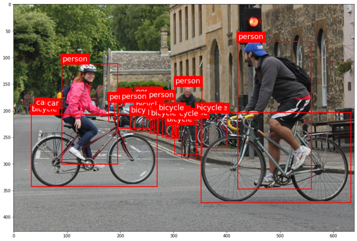
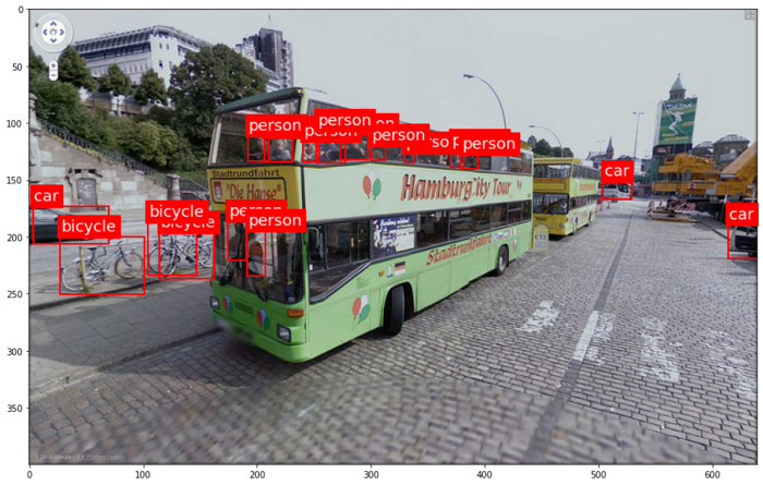
Below, you can find some samples from the training dataset. Each image contains multiple object annotations in the form of bounding boxes, denoted by their top-left corner coordinates (x, y) and their respective width and height (w, h).

YOLO model pipeline

Load the version YOLO network

To begin the YOLO detection process, we need to load the YOLO network. YOLO, which stands for You Only Look Once, is an incredibly fast algorithm for multi-object detection that leverages a convolutional neural network (CNN) to identify and localize objects.

In Python, I have created a pipeline for YOLO detection. To begin, we must download the pre-trained YOLO weight file and the YOLO configuration file. For this pipeline, I have chosen to use version v3 of YOLO.

The YOLO neural network consists of 254 elements, including convolutional layers (conv), rectified linear units (relu), and other components.

To load the YOLO model in Python, the following code snippet is used:

  net = cv.dnn.readNetFromDarknet('yolov3.cfg', 'yolov3.weights')

Create a blob

The input to the YOLO network is a blob object. To transform the image into a blob, we use the function cv.dnn.blobFromImage(img, scale, size, mean). This step is crucial as it involves preprocessing the data to ensure accurate predictions from the deep neural network.

The blobFromImage function performs the following operations:

• Resizing: It resizes the input image to a specific size required by the model. Deep learning models often have fixed input sizes, and the blobFromImage function ensures that the image is resized to match these requirements.

• Normalizing image: Dividing the image by 255 ensures that the pixel values are scaled between 0 and 1, can help ensure that gradients during the backpropagation process are within a reasonable range. This can aid in more stable and efficient convergence during training.

• Mean Subtraction: It subtracts the mean values from the image. Mean subtraction helps in normalizing the pixel values and removing the average color intensity. The mean values used for subtraction are usually pre-defined based on the dataset used to train the model.

• Channel Swapping: It reorders the color channels of the image. Deep learning models often expect images in a specific channel order, such as RGB (Red, Green, Blue). If the input image has a different channel order, the blobFromImage function swaps the channels accordingly.

In this case, the scale factor is set to 1/255, which ensures that the lightness of the image remains the same as the original.

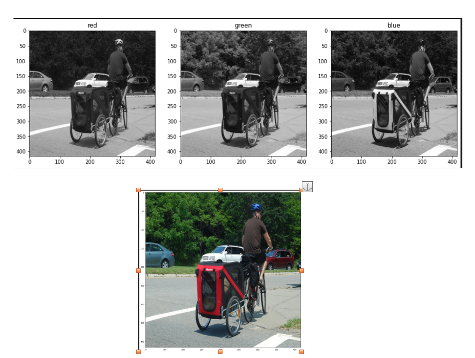
Once the image is transformed into a blob, it becomes a 4D NumPy array object with dimensions (images, channels, width, height) after resizing to (416, 416). The resulting blob consists of three channels: red, blue, and green. This can be visualized in the image below:

The blob object is then passed as input to the network, and the forward propagation is performed to retrieve all the layer names from the network and determine the output layers. The outputs object are vectors of length 85.

• 4x the predicted bounding box (centerx, centery, width, height)
• 1x box confidence: refers to the confidence score or probability assigned to the predicted bounding box. It represents the model's estimation of how confident it is that the bounding box accurately encloses an object in the image.
• 80x class confidence : these scores indicate the probabilities or confidences that an object detected in the image belongs to a particular class among 80 classes

Post processing

After obtaining the bounding boxes and their corresponding confidences from the output of an object detection model, it is common to apply a technique called Non-Maximum Suppression (NMS) to select the best bounding boxes.

NMS is a post-processing step that helps eliminate redundant or overlapping bounding box detections. Its purpose is to select the most accurate and representative bounding boxes while removing duplicates or highly overlapping detections.

In OpenCV, the cv.dnn.NMSBoxes() function is a convenient utility function that performs NMS. It accepts several parameters to fine-tune its behavior:

• boxes: This parameter represents the bounding boxes detected in the image. Each bounding box is typically represented as a list of four values (x, y, width, height) or as a tuple.

• confidences: This parameter contains the confidence scores associated with each bounding box. The confidence scores indicate the likelihood that the corresponding bounding box contains an object of interest.

• score_threshold: This parameter specifies the minimum confidence score threshold for considering a bounding box during NMS. Any bounding box with a confidence score below this threshold will be disregarded.

• nms_threshold: This parameter determines the overlap threshold for suppressing redundant bounding boxes. If the overlap between two bounding boxes exceeds this threshold, the one with the lower confidence score is suppressed.

The cv.dnn.NMSBoxes() function returns the indices of the selected bounding boxes that passed the NMS process. These indices correspond to the original list of bounding boxes and confidences, allowing you to access the selected boxes and their associated information.

Brainstorming: Multiple Options for Object Tagging in DigiKam

In this project, my goal is to empower users with the ability to choose specific options from a predefined set of 80 classes for automatic tagging in input images within DigiKam. We achieve this by leveraging the object detection capabilities of YOLO.

Let's take a look at an example from my research notebook, this picture include some objects like 'person', 'bike', 'car', 'bus':

After applying the YOLO model to the image, we obtain the following visualization with separated option from user:

Each image in the visualization represents a detected object, accompanied by a bounding box that highlights its location. This provides users with a clear understanding of the detected objects in the image.

In DigiKam, users have the freedom to select specific objects from the detected classes and assign appropriate tags to them. This flexibility allows for a personalized approach to organizing and categorizing images based on individual preferences and requirements.

(Week 3 - 4)

DONE

• Researched and created the Deeplearning pipeline to bencmark the different yolo version in term of the accuracy and inference time, decided which one should be intergrated into digiKam.
• Exported ONNX file for yoloVersion for the inference.
• Documentation

TODO

• Develop a mock widget in C++

Currently, In face engine, digiKam is using Yolov3 and SSD for recognition, the accuracy is better considering Yolov3. As a rough estimate, on a modern CPU, YOLOv3 can achieve around 1-2 FPS with an inference time of 500-1000 milliseconds per image. YOLOv4, being more computationally intensive, might have slightly lower performance on CPUs.

About object detection project, I actually benchmark this term for yolov3, for running through out 45 validation image, in order to calculate the average of the yolov3 and v4. And the inference time is the same as the estimate. Some evidences images, that I would like to show you.

Inference times and FPS YOLOv3 and YOLOv4 in CPU

YOLO version	Average Inference Times	Average FPS
YOLOV3	673.43ms	1.5 frames/s
YOLOV4	772.6	1.3 frames/s

It appears that YOLOv3 performs slightly better than YOLOv4 in terms of both inference time and FPS. YOLOv3 has a lower average inference time and a higher average FPS, indicating faster processing and better real-time performance compared to YOLOv4 on the tested CPU. YOLOv4 is generally considered to be a more advanced and complex model compared to YOLOv3. It introduces several architectural changes and additional components to improve accuracy and detection capabilities. However, these advancements may come at the cost of increased computational requirements, resulting in longer inference times and lower FPS.